Mastering the Many Models Approach

• Intro
• Setup
• Fundamentals
• Extensions
• Endgame
• Wrap-up
• Acknowledgements

Intro

The tidyverse “many models” approach was formally introduced in the first edition of R for Data Science (R4DS) in 2017. The central idea of this approach is to streamline the process of running the same model on various distinct subsets of data.

Since 2017, the tidyverse has evolved significantly, and along with it, the way we can harness the Many Models Approach. In this blog post we’ll first review the basic approach and update it using the latest tidyverse syntax. We’ll then explore a range of use cases with increasing complexity while introducing new building blocks and helper functions. This leads us finally up to the case where we not only run the same model on various, partly overlapping, subsets of our data, but where we also run slightly different models on those subsets simultaneously.

The structure of this blog post also reflects my motivation for writing it. I think that this is a powerful approach that should be more widely known. Those who are actually using it, often rely on an older syntax, which makes things more complicated than necessary. In addition to the original building blocks, there are several lesser-known functions that help apply this approach to more complex use cases.

Lately, the tidyverse Many Models Approach hasn’t received much attention. One might expect this to change with the release of the second edition of R4DS. However, the entire section on modeling has been omitted from this release. According to the authors, the reasons for this are twofold: First, there was never ample room to address the whole topic of modeling within R4DS. Second, the authors recommend the ‘tidymodels’ packages, which are well documented in Tidy Modeling with R and which should fill this gap.

While ‘tidymodels’ is a strong framework with definite advantages when working with various algorithms and model engines, it comes with considerable conceptual and syntactic overhead. For this reason, I believe there is still a lot room for the “classic” tidyverse Many Models Approach, which is based on ‘dplyr’ syntax but uses base R or alternatively package-specific models.

But before we delve into the use cases, let’s begin with the setup.

Setup

Unlike the name suggests, we don’t need all of the ‘tidyverse’ packages for the tidyverse Many Models Approach. The heavy lifting is done by ‘dplyr’ and ‘tidyr’. Additionally, we use ‘rlang’ and ‘purrr’ for some extra functionality. In this post we’ll be using the csat and csatraw data from my own package ‘dplyover’. It is important to note, that this post was written using ‘dplyr’ version 1.1.0. Readers who want to reproduce the code below should use at least ‘dplyr’ version version 1.0 or greater.

library(dplyr)        # <- necessary
library(tidyr)        # <- necessary
library(broom)        # <- necessary
library(rlang)        # <- nice to have
library(modelsummary) # <- for saving output
library(purrr)        # <- not really needed
library(dplyover)     # <- only for the data

csat is a mock-up dataset resembling data from a customer survey. It comes in two forms: the labeled data, csat, with meaningful column names and factor levels, and the corresponding raw data, csataw, where each column is a survey item and responses are just numbers. Since our models will be using the numbers instead of the factor levels, we’ll use the data from csatraw, but rename the columns according to csat (see my earlier post on how to rename variables). Additionally, we’ll drop variables that we don’t need. Let’s take a glimpse at the resulting dataset csat_named:

# create a look-up vector of old and new names
lookup_vec <- set_names(names(csatraw), names(csat))

# rename the columns
csat_named <- csatraw |>
  rename(any_of(lookup_vec)) |>
  select(cust_id, type, product, csat,
         ends_with("rating"))

glimpse(csat_named)
#> Rows: 150
#> Columns: 9
#> $ cust_id        <chr> "61297", "07545", "03822", "88219", "31831", "63646", "…
#> $ type           <chr> "existing", "existing", "existing", "reactivate", "new"…
#> $ product        <chr> "advanced", "advanced", "premium", "basic", "basic", "b…
#> $ csat           <dbl> 3, 2, 2, 4, 4, 3, 1, 3, 3, 2, 5, 4, 4, 1, 4, 4, 2, 3, 2…
#> $ postal_rating  <dbl> 3, 2, 5, 5, 2, NA, 3, 3, 4, NA, NA, 4, 3, 4, 1, 5, NA, …
#> $ phone_rating   <dbl> 2, 4, 5, 3, 5, 3, 4, 2, NA, 2, NA, NA, 2, 4, NA, 2, 4, …
#> $ email_rating   <dbl> NA, 3, NA, NA, 5, 2, 3, 5, 3, 1, 3, 1, 3, 1, 3, 3, 4, 1…
#> $ website_rating <dbl> 5, 2, 3, 4, 1, 3, 3, 1, 3, 2, 4, 2, NA, 4, 1, 2, NA, 5,…
#> $ shop_rating    <dbl> 3, 1, 2, 2, 5, 4, 4, 2, 2, 2, 4, 3, 2, NA, 3, 5, 4, 1, …

Every row is the response of a customer, cust_id, who owns a contract-base product available in different flavors: “basic”, “advanced” or “premium”. There are three different types of customers: “existing”, “new” and “reactivate”. Our dependent variable is the customer satisfaction score, csat, which ranges from ‘1 = Very unsatisfied’ to ‘5 = Very satisfied’. The independent variables are ratings on the same scale concerning the following touchpoints: “postal”, “phone”, “email”, “website” and “shop”. We’ve dropped all other variables, but interested readers can find both datasets well documented in the ‘dplyover’ package ( ?csat, ?csatraw).

Fundamentals

Let’s start with the basic approach as it was introduced in R4DS. Keep in mind that syntax and functions have evolved over the past five years, so we’ll be refining the original ideas into a more canonical form.

Before we dive into the details let’s look at the whole workflow from a computational perspective. We start by breaking down our original data into small grouped subsets, where each data set is stored in a row of a so called “nested” data.frame. The model fitting function is applied iteratively to each row. The model fits are appended to a new column of the nested data frame, again, one summary per row. We further process and tidy the results by turning the original model output into a list of small data.frames which can also be appended to a new column. Finally, we concatenate the small data.frames in each row and turn them into one big unified data.frame holding the results of all subgroups.

There are four essential components in the workflow above that we’ll be discussing in detail below:

1. nested data
2. rowwise operations
3. tidy results
4. unnesting results

If you’re already familiar with these concepts, feel free to skip this section.

Nested data

The central idea of the Many Models Approach is to streamline the process of running models on various subsets of data. Let’s say we want to perform a linear regression on each product type. In a traditional base R approach, we might have used a for loop to populate a list object with the results of each run. However, the tidyverse method begins with a nested data.frame.

So, what is a nested data.frame? We can use dplyr::nest_by(product) to create a data.frame containing three rows, one for each product. The second column, data, is a ‘list-column’ that holds a list of data.frame's—one for each row. These data.frames contain data for all customers within the corresponding product category. If you’re unfamiliar with list-columns, I highly recommend reading chapter 25 of R4DS. Although some parts may be outdated, it remains an excellent resource for understanding the essential components of this approach.

csat_prod_nested <- csat_named |>
  nest_by(product) 

csat_prod_nested
#> # A tibble: 3 × 2
#> # Rowwise:  product
#>   product                data
#>   <chr>    <list<tibble[,8]>>
#> 1 advanced           [40 × 8]
#> 2 basic              [60 × 8]
#> 3 premium            [50 × 8]

Looking at the first element (row) of the data column shows a data.frame with 40 customers, all of whom have “advanced” products. The product column is omitted, as this information is already included in our nested data: csat_prod_nested.

csat_prod_nested$data[[1]]
#> # A tibble: 40 × 8
#>    cust_id type        csat postal_rating phone_rating email_r…¹ websi…² shop_…³
#>    <chr>   <chr>      <dbl>         <dbl>        <dbl>     <dbl>   <dbl>   <dbl>
#>  1 61297   existing       3             3            2        NA       5       3
#>  2 07545   existing       2             2            4         3       2       1
#>  3 63600   existing       1             3            4         3       3       4
#>  4 82048   reactivate     3             3            2         5       1       2
#>  5 41142   reactivate     3             4           NA         3       3       2
#>  6 06387   reactivate     1             4            4         1       4      NA
#>  7 63024   existing       2            NA            4         4      NA       4
#>  8 55743   new            1             4            5         4       1       5
#>  9 32689   new            5             3           NA         3       4       2
#> 10 33603   existing       2             3            3         4       3       2
#> # … with 30 more rows, and abbreviated variable names ¹​email_rating,
#> #   ²​website_rating, ³​shop_rating

Rowwise operations

Applying nest_by() also groups our data rowwise(). This means that subsequent dplyr operations will be applied “one row at a time.” This is particularly helpful when vectorized functions aren’t available, such as the lm() function in our case, which we want to apply to the data in each row.

First, let’s define the relationship between our dependent and independent variables using a formula object, base_formula.

base_formula <- csat ~ postal_rating + phone_rating + email_rating +
  website_rating + shop_rating

base_formula
#> csat ~ postal_rating + phone_rating + email_rating + website_rating + 
#>     shop_rating

Note, that this is a basic “model formula” which holds the dependent variable, csat, on the left-hand side (of the tilde ~) and all independent variables on the right-hand side.

Next, we use mutate to create new columns. We’ll start by creating a column called mod containing our model. We’ll apply the lm() function with the previously defined formula and supply the data column to it. Note, that when supplying arguments within dplyr::mutate() we can use both: (i) objects from the data.frame we are working on, here the data column of our csat_prod_nested dataset, and (ii) objects from the enclosing environment, here the global environment, where our formula object base_formula resides.

Since we are working with a rowwise data.frame, the lm() function is executed three times, one time for each row, each time using a different data.frame in the list-column data. As the result of each call is not an atomic vector, but an lm object of type list, we need to wrap the function call in list(). This results in a new list-column, mod, which holds an lm object in each row.

csat_prod_nested |>
  mutate(mod = list(lm(base_formula, data = data)))
#> # A tibble: 3 × 3
#> # Rowwise:  product
#>   product                data mod   
#>   <chr>    <list<tibble[,8]>> <list>
#> 1 advanced           [40 × 8] <lm>  
#> 2 basic              [60 × 8] <lm>  
#> 3 premium            [50 × 8] <lm>

Two notes of caution when using dplyr::rowwise():

First, keep in mind that we need the wrapping list() call whenever the result is not an atomic vector. Since this is fairly often the case, it’s good practice to resonate about the return type of a function when using dplyr::rowwise().

Second, once we call rowwise() on a data.frame(), all following operations will be applied row-by-row. We can revoke this by calling ungroup() on a rowwise data.frame. Sometimes we might forget to ungroup(). In most cases this will not lead to an error. However, it will lead to a degraded performance, since vectorized functions, which are supposed to work on whole columns, are now unnecessarily applied row-by-row.

Tidy results with broom

To make the results of this model more accessible, we’ll use two functions from the ‘broom’ package:

broom::glance() returns a data.frame containing all model statics, such as r-squared, BIC, AIC etc., and the overall p-value of the model itself.

broom::tidy() returns a data.frame with all regression terms, their estimates, p-values and other statistics.

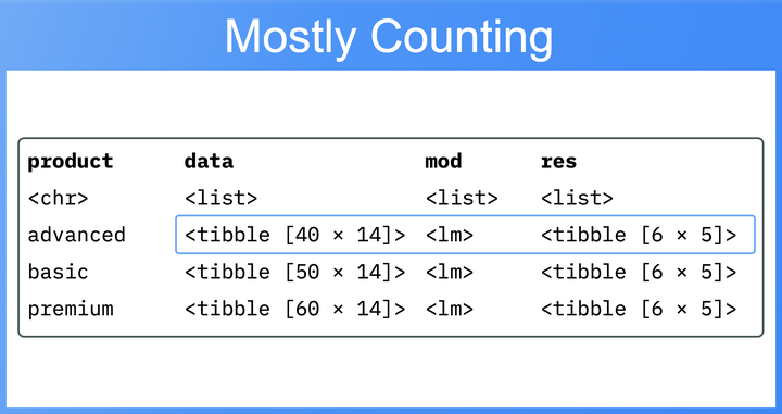
Again, we’ll wrap both functions in list() and call them on the model in the new mod column. This yields a final, nested data.frame. The rows represent the three product subgroups, while the columns contain the input data, the model mod, and the results modstat and res. Beside mod, each of these columns is a list of data.frames:

csat_prod_nested_res <- csat_prod_nested |>
  mutate(mod     = list(lm(base_formula, data = data)),
         modstat = list(broom::glance(mod)),
         res =     list(broom::tidy(mod)))

csat_prod_nested_res
#> # A tibble: 3 × 5
#> # Rowwise:  product
#>   product                data mod    modstat           res             
#>   <chr>    <list<tibble[,8]>> <list> <list>            <list>          
#> 1 advanced           [40 × 8] <lm>   <tibble [1 × 12]> <tibble [6 × 5]>
#> 2 basic              [60 × 8] <lm>   <tibble [1 × 12]> <tibble [6 × 5]>
#> 3 premium            [50 × 8] <lm>   <tibble [1 × 12]> <tibble [6 × 5]>

Unnesting results

With the groundwork laid, it is now easy to access the results. To do this, we’ll use tidyr::unnest() to convert a list of data.frames back into a regular data.frame. First, lets look at the model statistics. We’ll select the product and modstat columns and unnest the latter. This produces a data.frame with different model statistics for the three product subgroups. In this case, we’re interested in the r-squared, the p-value and the number of observations of each model:

csat_prod_nested_res |>
  select(product, modstat) |>
  unnest(modstat) |>
  select(r.squared, p.value, nobs)
#> Adding missing grouping variables: `product`
#> # A tibble: 3 × 4
#> # Groups:   product [3]
#>   product  r.squared p.value  nobs
#>   <chr>        <dbl>   <dbl> <int>
#> 1 advanced     0.112   0.941    15
#> 2 basic        0.382   0.192    20
#> 3 premium      0.185   0.645    21

Please note that the results themselves aren’t the main focus here, as the primary goal is to demonstrate how the approach works in general.

Next, we’ll inspect the coefficients, their size and their p-values. We’ll select the product and res columns and unnest the latter. Additionally, since we’re not interested in the size of the intercept, we’ll filter out those rows.

csat_prod_nested_res |>
  select(product, res) |>
  unnest(res) |>
  filter(term != "(Intercept)")
#> # A tibble: 15 × 6
#> # Groups:   product [3]
#>    product  term           estimate std.error statistic p.value
#>    <chr>    <chr>             <dbl>     <dbl>     <dbl>   <dbl>
#>  1 advanced postal_rating   0.396       0.483   0.819     0.434
#>  2 advanced phone_rating   -0.235       0.423  -0.556     0.592
#>  3 advanced email_rating    0.349       0.485   0.720     0.490
#>  4 advanced website_rating  0.398       0.456   0.874     0.405
#>  5 advanced shop_rating    -0.00183     0.288  -0.00637   0.995
#>  6 basic    postal_rating  -0.324       0.225  -1.44      0.172
#>  7 basic    phone_rating   -0.297       0.237  -1.25      0.231
#>  8 basic    email_rating   -0.136       0.249  -0.547     0.593
#>  9 basic    website_rating  0.229       0.229   1.00      0.334
#> 10 basic    shop_rating     0.321       0.259   1.24      0.235
#> 11 premium  postal_rating   0.0538      0.220   0.245     0.810
#> 12 premium  phone_rating   -0.508       0.307  -1.65      0.119
#> 13 premium  email_rating    0.375       0.309   1.22      0.243
#> 14 premium  website_rating -0.175       0.259  -0.677     0.509
#> 15 premium  shop_rating     0.0498      0.203   0.246     0.809

From this point, we could further manipulate the resulting data, such as filtering out non-significant coefficients or plotting the model results, and so on.

To wrap up this section, the info box below highlights how the approach above deviates from the original syntax introduced in R4DS.

csat_named |>
  group_by(product) |>
  nest() |>
  ungroup() |>
  mutate(mod     = map(data, ~ lm(base_formula, data = .x)),
         res     = map(mod, broom::tidy),
         modstat = map(mod, broom::glance))
#> # A tibble: 3 × 5
#>   product  data              mod    res              modstat          
#>   <chr>    <list>            <list> <list>           <list>           
#> 1 advanced <tibble [40 × 8]> <lm>   <tibble [6 × 5]> <tibble [1 × 12]>
#> 2 premium  <tibble [50 × 8]> <lm>   <tibble [6 × 5]> <tibble [1 × 12]>
#> 3 basic    <tibble [60 × 8]> <lm>   <tibble [6 × 5]> <tibble [1 × 12]>

Extensions

Building on the basic approach outlined above, we’ll introduce six advanced building blocks that help to tackle more complex use cases.

1. create an overall category with bind_rows()
2. add subgroups through filters with expand_grid()
3. dynamically name list elements with rlang::list2()
4. use data-less grids
5. build formulas programmatically with reformulate()
6. save model output to Excel with modelsummary()

Create an overall category with ‘bind_rows()’

Often we want to run an analysis not only on different subsets of the data but also on the entire dataset simultaneously. We can achieve this by using mutate() and bind_rows() to create an additional overall product category that encompasses all products.

csat_all <- csat_named |>
  mutate(product = "All") |>
  bind_rows(csat_named) 

csat_all |> count(product)
#> # A tibble: 4 × 2
#>   product      n
#>   <chr>    <int>
#> 1 All        150
#> 2 advanced    40
#> 3 basic       60
#> 4 premium     50

First, we use mutate() to overwrite the ‘product’ column with the value “All” effectively grouping all products together under this new label. We then use bind_rows() to merge the original csat_named dataset with the modified dataset from the previous step. This results in a new dataset called csat_all that contains the original data and an extra set of rows where the product category is labeled as “All”. Consequently, the new dataset is twice the size of the original data, as it includes each row twice.

Now we can apply the same analysis as above:

csat_all |>
  nest_by(product) |>
  mutate(mod     = list(lm(base_formula, data = data)),
         res     = list(broom::tidy(mod)),
         modstat = list(broom::glance(mod)))

#> # A tibble: 4 × 5
#> # Rowwise:  product
#>   product                data mod    res              modstat          
#>   <chr>    <list<tibble[,8]>> <list> <list>           <list>           
#> 1 All               [150 × 8] <lm>   <tibble [6 × 5]> <tibble [1 × 12]>
#> 2 advanced           [40 × 8] <lm>   <tibble [6 × 5]> <tibble [1 × 12]>
#> 3 basic              [60 × 8] <lm>   <tibble [6 × 5]> <tibble [1 × 12]>
#> 4 premium            [50 × 8] <lm>   <tibble [6 × 5]> <tibble [1 × 12]>

Add subgroups through filters with ‘expand_grid()’

Sometimes, we may want to create additional subgroups that meet specific filter criteria. For instance, we might want to analyze all customers and, at the same time, compare the results with an analysis of all customers who are not of the “reactivate” type.

To achieve this, we’ll follow three steps:

1. We create a list of filter expressions, referred to as filter_ls.

   filter_ls <- list(
     All = TRUE,
     no_reactivate = expr(type != "reactivate")
   )
   
   filter_ls
   #> $All
   #> [1] TRUE
   #> 
   #> $no_reactivate
   #> type != "reactivate"
   

   This results in a list where each element is either TRUE or an unevaluated expression that we’ll use later inside filter(). Note that we use rlang::expr() to capture an expression, although we could have used substitute() or quote() instead. Omitting any of these function would result in an error, as R would try to evaluate type which is not desired since we want to delay the evaluation until later.

2. We expand our nested data.frame for each filter category using expand_grid().

   csat_all_grps <- csat_all |>
     nest_by(product) |>
     expand_grid(filter_ls) |>
     mutate(type = names(filter_ls),
            .after = product)
   
   csat_all_grps
   #> # A tibble: 8 × 4
   #>   product  type                        data filter_ls   
   #>   <chr>    <chr>         <list<tibble[,8]>> <named list>
   #> 1 All      All                    [150 × 8] <lgl [1]>   
   #> 2 All      no_reactivate          [150 × 8] <language>  
   #> 3 advanced All                     [40 × 8] <lgl [1]>   
   #> 4 advanced no_reactivate           [40 × 8] <language>  
   #> 5 basic    All                     [60 × 8] <lgl [1]>   
   #> 6 basic    no_reactivate           [60 × 8] <language>  
   #> 7 premium  All                     [50 × 8] <lgl [1]>   
   #> 8 premium  no_reactivate           [50 × 8] <language>
   

   We use tidyr::expand_grid() to expand our nested data for each category in our list of filter expressions: filter_ls. expand_grid() creates a tibble from all combinations of the supplied objects—this can be any mix of atomic vectors, lists or data.frames. Note that in the case of the latter, all groupings are ignored. Looking at the output reveals that our original nested data.frame contained four rows, while our data now holds eight rows - one for each combination of product and type.

   We also use dplyr::mutate() to add a new column, type, to actually show which row refers to which type. The names() of our list column filter_ls contain this information. To show the type next to the product column we use the argument .after in mutate(). Without specifying this, the type column would have been added as the last column in our nested data.frame.

3. We apply each filter to our data rowwise using dplyr::filter(eval(filter_ls)).

   csat_all_grps_grid <- csat_all_grps |>
     rowwise() |>
     mutate(data = list(
       filter(data, eval(filter_ls))
       ),
       .keep = "unused"
     )
   
   csat_all_grps_grid
   #> # A tibble: 8 × 3
   #> # Rowwise: 
   #>   product  type          data              
   #>   <chr>    <chr>         <list>            
   #> 1 All      All           <tibble [150 × 8]>
   #> 2 All      no_reactivate <tibble [120 × 8]>
   #> 3 advanced All           <tibble [40 × 8]> 
   #> 4 advanced no_reactivate <tibble [32 × 8]> 
   #> 5 basic    All           <tibble [60 × 8]> 
   #> 6 basic    no_reactivate <tibble [46 × 8]> 
   #> 7 premium  All           <tibble [50 × 8]> 
   #> 8 premium  no_reactivate <tibble [42 × 8]>
   

   We use mutate to apply filter() to each data.frame in the data column in each row. As filter expression we use the column filter_ls and evaluate it. Since we no longer need this column, we set the .keep argument in mutate to “unused” to eventually drop filter_ls after it has been used.

From this point, we could continue applying our model and then calculating and extracting the results, but we’ll omit this for the sake of brevity.

csat_all_grps_grid <- csat_all_grps |>
  rowwise() |>
  mutate(mod = list(lm(base_formula, data = data)),
         res = list(broom::tidy(mod)),
         modstat = list(broom::glance(mod)))

csat_all_grps_grid |>
  select(product, type, modstat) |>
  unnest(modstat) |>
  select(-c(sigma, statistic, df:df.residual))
#> # A tibble: 8 × 6
#>   product  type          r.squared adj.r.squared p.value  nobs
#>   <chr>    <chr>             <dbl>         <dbl>   <dbl> <int>
#> 1 All      All               0.134        0.0479   0.191    56
#> 2 All      no_reactivate     0.134        0.0479   0.191    56
#> 3 advanced All               0.112       -0.381    0.941    15
#> 4 advanced no_reactivate     0.112       -0.381    0.941    15
#> 5 basic    All               0.382        0.161    0.192    20
#> 6 basic    no_reactivate     0.382        0.161    0.192    20
#> 7 premium  All               0.185       -0.0867   0.645    21
#> 8 premium  no_reactivate     0.185       -0.0867   0.645    21

csat_all_grps_grid |>
  select(product, type, res) |>
  unnest(res) |>
  filter(term == "website_rating")
#> # A tibble: 8 × 7
#>   product  type          term           estimate std.error statistic p.value
#>   <chr>    <chr>         <chr>             <dbl>     <dbl>     <dbl>   <dbl>
#> 1 All      All           website_rating   0.0729     0.141     0.517   0.607
#> 2 All      no_reactivate website_rating   0.0729     0.141     0.517   0.607
#> 3 advanced All           website_rating   0.398      0.456     0.874   0.405
#> 4 advanced no_reactivate website_rating   0.398      0.456     0.874   0.405
#> 5 basic    All           website_rating   0.229      0.229     1.00    0.334
#> 6 basic    no_reactivate website_rating   0.229      0.229     1.00    0.334
#> 7 premium  All           website_rating  -0.175      0.259    -0.677   0.509
#> 8 premium  no_reactivate website_rating  -0.175      0.259    -0.677   0.509

Although this example is relatively simple, it demonstrates how this approach can be significantly expanded by providing more filter expressions in our filter_ls list or by using multiple lists of filter expressions. This is particularly useful when performing robustness checks, where we attempt to reproduce the original findings on specific subgroups of our data.

Dynamically name list elements with ‘rlang::list2()’

So far, we’ve wrapped the results of our rowwise operations in list() when they produced non-atomic vectors.

A common issue when inspecting the results is that these list-columns are often unnamed, making it difficult to determine which element we’re examining. For instance, suppose that we want to double-check the output of our call to broom::glance(mod) stored in the modstat column. Let’s look at the fourth element:

csat_all_grps_grid$modstat[4]
#> [[1]]
#> # A tibble: 1 × 12
#>   r.squ…¹ adj.r…² sigma stati…³ p.value    df logLik   AIC   BIC devia…⁴ df.re…⁵
#>     <dbl>   <dbl> <dbl>   <dbl>   <dbl> <dbl>  <dbl> <dbl> <dbl>   <dbl>   <int>
#> 1   0.112  -0.381  1.39   0.228   0.941     5  -22.4  58.9  63.8    17.5       9
#> # … with 1 more variable: nobs <int>, and abbreviated variable names
#> #   ¹​r.squared, ²​adj.r.squared, ³​statistic, ⁴​deviance, ⁵​df.residual

The result prints nicely, but it’s unclear which subset of the data it belongs to.

Here rlang::list2() comes to the rescue. Although it resembles list(), it provides some extra functionality. Specifically, it allows us to unquote names on the left-hand side of the walrus operator. To better grasp this idea, let’s look at an example.

We wrap our calls to lm(), tidy() and glance() in list2() and name each element using the walrus operator :=. On the left-hand side of the walrus operator, we use the glue operator { within a string to dynamically name each element according to the values in the product and type columns in each row. When we inspect the fourth element of the modstat column, we can quickly see that these model statistics belong to the subset of customers with an “advanced” product and who are not of type “reactivate”.

csat_all_grps_grid <- csat_all_grps |>
  rowwise() |>
  mutate(mod     = list2("{product}_{type}" := lm(base_formula, data = data)),
         res     = list2("{product}_{type}" := broom::tidy(mod)),
         modstat = list2("{product}_{type}" := broom::glance(mod)))

csat_all_grps_grid$modstat[4]
#> $advanced_no_reactivate
#> # A tibble: 1 × 12
#>   r.squ…¹ adj.r…² sigma stati…³ p.value    df logLik   AIC   BIC devia…⁴ df.re…⁵
#>     <dbl>   <dbl> <dbl>   <dbl>   <dbl> <dbl>  <dbl> <dbl> <dbl>   <dbl>   <int>
#> 1   0.112  -0.381  1.39   0.228   0.941     5  -22.4  58.9  63.8    17.5       9
#> # … with 1 more variable: nobs <int>, and abbreviated variable names
#> #   ¹​r.squared, ²​adj.r.squared, ³​statistic, ⁴​deviance, ⁵​df.residual

Data-less grids

Using the methods described above, we can easily construct nested data.frames with several dozens of subgroups. However, this approach can be inefficient in terms of memory usage, as we create a copy of our data for every single subgroup. To make this approach more memory-efficient, we can use what I call a “data-less grid”, which is similar to our original nested data.frame, but without the data column.

Instead of nesting our data with nest_by(), we manually create the combinations of subgroups to which we want to apply our model. We start with a vector of all unique values in the product column and add an overall category “All” to it. Then, we supply this vector along with our list of filter expressions filter_ls to expand_grid(). Finally, we place the names of the elements in filter_ls in a separate column: type.

This results in an initial grid all_grps_grid of combinations between product and type, with an additional column of filter expressions.

product <- c(
  "All", unique(csat_named$product)
)

all_grps_grid <- expand_grid(product, filter_ls) |>
  mutate(type = names(filter_ls),
         .after = product)

all_grps_grid
#> # A tibble: 8 × 3
#>   product  type          filter_ls   
#>   <chr>    <chr>         <named list>
#> 1 All      All           <lgl [1]>   
#> 2 All      no_reactivate <language>  
#> 3 advanced All           <lgl [1]>   
#> 4 advanced no_reactivate <language>  
#> 5 premium  All           <lgl [1]>   
#> 6 premium  no_reactivate <language>  
#> 7 basic    All           <lgl [1]>   
#> 8 basic    no_reactivate <language>

The challenging aspect here is to generate each data subset on the fly in the call to lm(). To accomplish this, we filter() our initial data csat_named on two conditions:

1. Firstly, we filter for different product types using an advanced filter expression:

   .env$product == "All" | .env$product == product.

   This expression may appear somewhat obscure, so let’s break it down:

   The issue here is that both our original data csat_named and our grid all_grps_grid contain a column named product. By default, product, in the filter() call below, refers to the column in csat_named. To tell ‘dyplr’ to use the column in our grid all_grps_grid we use the .env pronoun.

   So, the filter expression above essentially states: If the product category in our grid .env$product is “All”, then select all rows. This works because when the left side of the or-condition .env$product == "All" evaluates to TRUE, filter selects all rows. If the first part of our condition is not true, then the product column in csat_named should match the value of the product column of our data-less grid .env$product.

2. Next, we filter the different types of customers. Here, we use the filter expressions stored in filter_ls and evaluate them. Since we don’t need the filter_ls column after we’ve used it to create the data column, we just drop it with select(! filter_ls):

all_grps_grid_mod <- all_grps_grid |>
  rowwise() |>
  mutate(mod = list(
    lm(base_formula,
       data = filter(csat_named,
                     # 1. filter product categories
                     .env$product == "All" | .env$product == product,
                     
                     # 2. filter customer types
                     eval(filter_ls) 
                     )
       )
    )
    ) |>
  select(! filter_ls)

all_grps_grid_mod
#> # A tibble: 8 × 3
#> # Rowwise: 
#>   product  type          mod   
#>   <chr>    <chr>         <list>
#> 1 All      All           <lm>  
#> 2 All      no_reactivate <lm>  
#> 3 advanced All           <lm>  
#> 4 advanced no_reactivate <lm>  
#> 5 premium  All           <lm>  
#> 6 premium  no_reactivate <lm>  
#> 7 basic    All           <lm>  
#> 8 basic    no_reactivate <lm>

This returns our initial grid, now extended by an additional column, mod, containing the linear models.

The remaining steps do not significantly differ from our initial approach, so we will omit them for brevity.

all_grps_grid_res <- all_grps_grid_mod |>
  mutate(res     = list(broom::tidy(mod)),
         modstat = list(broom::glance(mod))) 

all_grps_grid_res |>
  select(product, type, modstat) |>
  unnest(modstat) |>
  select(-c(sigma, statistic, df:df.residual))
#> # A tibble: 8 × 6
#>   product  type          r.squared adj.r.squared p.value  nobs
#>   <chr>    <chr>             <dbl>         <dbl>   <dbl> <int>
#> 1 All      All               0.134        0.0479   0.191    56
#> 2 All      no_reactivate     0.180        0.0771   0.145    46
#> 3 advanced All               0.112       -0.381    0.941    15
#> 4 advanced no_reactivate     0.330       -0.340    0.772    11
#> 5 premium  All               0.185       -0.0867   0.645    21
#> 6 premium  no_reactivate     0.156       -0.196    0.810    18
#> 7 basic    All               0.382        0.161    0.192    20
#> 8 basic    no_reactivate     0.465        0.221    0.172    17

Build formulas programmatically with ‘reformulate’

One last major building block that essentially completes the Many Models Approach is actually a base R function: reformulate().

I recently posted an #RStats meme on Twitter highlighting that reformulate() is one of the lesser-known base R functions, even among advanced users. The reactions to my post largely confirmed my impression.

Before applying reformulate() in the many models context, let’s have a look at what it does. Instead of manually creating a formula object by typing y ~ x1 + x2, we can use reformulate() to generate a formula object based on character vectors.

Important is the order of the first two arguments. While we start writing a formula from the left-hand side y, reformulate() takes as first argument the right-hand side. We could, of course, change the order and call the arguments by name instead of position, but I wouldn’t recommend this, because it might confuse readers. Nevertheless, calling the arguments by name, termlabels and response, and their correct position is a good idea to make clear which is which and to remind readers that the argument order is different to what they might expect.

form1 <- y ~ x1 + x2
form1 
#> y ~ x1 + x2

form2 <- reformulate(termlabels = c("x1", "x2"),
                     response = "y")
form2
#> y ~ x1 + x2

identical(form1, form2)
#> [1] TRUE

How can we make use of reformulate() in the Many Models Approach?

In the following we’ll look at two use cases. The first use case covers a situation where we need to fit multiple models to the data in each row of a nested data frame. All of these models share the same response variable and we use reformulate() to supply different predictor variables in each iteration. The second use case covers a situation where we also need to fit multiple models to the data in each row of a nested data frame. However, this time we define a base model in advance and add different variables on top of it in each iteration.

Let’s begin with the first use case outline above in which we want to construct a separate model for each independent variable, containing only our response variable and one independent variable at a time: csat ~ indepedent_variable. And of course, we want to do this for all of our subgroups of the previous approach.

First, we need a character vector holding the names of our independent variables. With this vector, we can now expand our data-less grid from above. This results in a new grid with 40 rows (eight subgroups times five independent variables).

indep_vars <- c("postal_rating",
                "phone_rating",
                "email_rating",
                "website_rating",
                "shop_rating")

all_grps_grid_vars <- all_grps_grid |>
   expand_grid(indep_vars)

all_grps_grid_vars
#> # A tibble: 40 × 4
#>    product type          filter_ls    indep_vars    
#>    <chr>   <chr>         <named list> <chr>         
#>  1 All     All           <lgl [1]>    postal_rating 
#>  2 All     All           <lgl [1]>    phone_rating  
#>  3 All     All           <lgl [1]>    email_rating  
#>  4 All     All           <lgl [1]>    website_rating
#>  5 All     All           <lgl [1]>    shop_rating   
#>  6 All     no_reactivate <language>   postal_rating 
#>  7 All     no_reactivate <language>   phone_rating  
#>  8 All     no_reactivate <language>   email_rating  
#>  9 All     no_reactivate <language>   website_rating
#> 10 All     no_reactivate <language>   shop_rating   
#> # … with 30 more rows

We can now apply a similar approach as before, creating data subgroups on the fly. The only change is that we use reformulate(indep_vars, "csat") instead of our formula object base_formula. This adds forty different linear models to our grid:

all_grps_grid_vars_mod <- all_grps_grid_vars |>

  rowwise() |>

  mutate(mod = list(
    lm(reformulate(indep_vars, "csat"), # <- this part is new
       data = filter(csat_named,
                     .env$product == "All" | .env$product == product,
                     eval(filter_ls)
       )
    )
  )
  ) %>%
  select(! filter_ls)

all_grps_grid_vars_mod
#> # A tibble: 40 × 4
#> # Rowwise: 
#>    product type          indep_vars     mod   
#>    <chr>   <chr>         <chr>          <list>
#>  1 All     All           postal_rating  <lm>  
#>  2 All     All           phone_rating   <lm>  
#>  3 All     All           email_rating   <lm>  
#>  4 All     All           website_rating <lm>  
#>  5 All     All           shop_rating    <lm>  
#>  6 All     no_reactivate postal_rating  <lm>  
#>  7 All     no_reactivate phone_rating   <lm>  
#>  8 All     no_reactivate email_rating   <lm>  
#>  9 All     no_reactivate website_rating <lm>  
#> 10 All     no_reactivate shop_rating    <lm>  
#> # … with 30 more rows

Note, that we again drop the filter_ls column after we used it to create out data.

Although the example above is instructive, it isn’t particularly useful. In most cases, we don’t want to create a separate model for each independent variable. A much more powerful way to use reformulate() is to update() a baseline model with additional variables. So let’s look at our second use case.

Assume we have the following minimal version of our base-line model:

min_formula <- csat ~ postal_rating + phone_rating + shop_rating
min_formula
#> csat ~ postal_rating + phone_rating + shop_rating

For our many subgroups from above, we want to check if adding (i) email_rating or (ii) website_rating or (iii) both variables at once, or (iv) both variables and their interaction effect, improve our model. Let’s create a list of terms that we want to add to our model: update_vars.

update_vars <- list(base = NULL,
                    email = "email_rating",
                    website = "website_rating",
                    both = c("email_rating", "website_rating"),
                    both_plus_interaction = "email_rating*website_rating")

There are two noteworthy aspects here. First, we need to include NULL, as this will represent our baseline model without any additional variables. Second, we are not limited to plain variable names as strings. We can even include interaction effects using the same notation that the tilde operator supports, that is by adding an asterisk * between two variable names.

Now we expand our grid from above with this list and put the names of each variable (“base”, “email”, “website” etc.) in a separate column to keep track of which model we are examining.

all_grid_upd_vars <- all_grps_grid |>
  expand_grid(update_vars) |>
  mutate(model_spec = names(update_vars),
         .after = type)

all_grid_upd_vars
#> # A tibble: 40 × 5
#>    product type          model_spec            filter_ls    update_vars 
#>    <chr>   <chr>         <chr>                 <named list> <named list>
#>  1 All     All           base                  <lgl [1]>    <NULL>      
#>  2 All     All           email                 <lgl [1]>    <chr [1]>   
#>  3 All     All           website               <lgl [1]>    <chr [1]>   
#>  4 All     All           both                  <lgl [1]>    <chr [2]>   
#>  5 All     All           both_plus_interaction <lgl [1]>    <chr [1]>   
#>  6 All     no_reactivate base                  <language>   <NULL>      
#>  7 All     no_reactivate email                 <language>   <chr [1]>   
#>  8 All     no_reactivate website               <language>   <chr [1]>   
#>  9 All     no_reactivate both                  <language>   <chr [2]>   
#> 10 All     no_reactivate both_plus_interaction <language>   <chr [1]>   
#> # … with 30 more rows

We could use update() directly in our call to lm(), but to avoid overcomplicating things, let’s create a column holding our updated formula, form, and use that in our call to lm():

all_grid_upd_vars_form <- all_grid_upd_vars |>

  rowwise() |>

  mutate(
    form = list(
      update(
        min_formula, # old formula
        reformulate(c(".", update_vars)) # changes to formula
        )
      ),

    mod = list2( "{product}_{type}_{model_spec}" :=
    lm(form,
       data = filter(csat_named,
                     .env$product == "All" | .env$product == product,
                     eval(filter_ls)
                     )
       )
    )
  )

update() takes two arguments, the formula we want to update, in this case min_formula, and the formula we use to update the former. In our case, this is a call to reformulate() which says: “take all the original term labels ".", and add c() to them the variable in update_vars. Now its probably clear why we included NULL in update_vars. In cases where it is NULL the original formula won’t be updated, which corresponds to our baseline model.

Checking the first five rows of our list-column containing the model shows that the approach works as intended:

head(all_grid_upd_vars_form$mod, 5)

#> $All_All_base
#> 
#> Call:
#> lm(formula = form, data = filter(csat_named, .env$product == 
#>     "All" | .env$product == product, eval(filter_ls)))
#> 
#> Coefficients:
#>   (Intercept)  postal_rating   phone_rating    shop_rating  
#>       4.08357        0.02305       -0.26742       -0.11736  
#> 
#> 
#> $All_All_email
#> 
#> Call:
#> lm(formula = form, data = filter(csat_named, .env$product == 
#>     "All" | .env$product == product, eval(filter_ls)))
#> 
#> Coefficients:
#>   (Intercept)  postal_rating   phone_rating    shop_rating   email_rating  
#>       4.21064       -0.01306       -0.35218       -0.01432        0.01203  
#> 
#> 
#> $All_All_website
#> 
#> Call:
#> lm(formula = form, data = filter(csat_named, .env$product == 
#>     "All" | .env$product == product, eval(filter_ls)))
#> 
#> Coefficients:
#>    (Intercept)   postal_rating    phone_rating     shop_rating  website_rating  
#>        3.59965        -0.03583        -0.22622        -0.04578         0.13008  
#> 
#> 
#> $All_All_both
#> 
#> Call:
#> lm(formula = form, data = filter(csat_named, .env$product == 
#>     "All" | .env$product == product, eval(filter_ls)))
#> 
#> Coefficients:
#>    (Intercept)   postal_rating    phone_rating     shop_rating    email_rating  
#>        3.72401        -0.05946        -0.36126         0.05673         0.10789  
#> website_rating  
#>        0.07286  
#> 
#> 
#> $All_All_both_plus_interaction
#> 
#> Call:
#> lm(formula = form, data = filter(csat_named, .env$product == 
#>     "All" | .env$product == product, eval(filter_ls)))
#> 
#> Coefficients:
#>                 (Intercept)                postal_rating  
#>                     3.46609                     -0.05549  
#>                phone_rating                  shop_rating  
#>                    -0.36445                      0.05816  
#>                email_rating               website_rating  
#>                     0.18616                      0.15469  
#> email_rating:website_rating  
#>                    -0.02658

Save model output to Excel with ‘modelsummary()’

Although we previously used the ‘broom’ package to create tidy data.frames containing the model statistics, modstat created with broom::glance(), and the model results, res created with broom::tidy(), we ideally need both pieces of information when exporting the model output to Excel (or any other spreadsheet).

In this case, the modelsummary() function from the package of the same name proves extremely helpful. It creates an Excel file that includes both model statistics and estimator results, which is convenient when reporting our model findings to a non-R-user audience.

The great feature of modelsummary() is that it accepts list-columns of model objects, such as our mod column containing many lm objects, as input. We can specify various output formats—below we choose ".xlsx". Numerous other arguments allow us to trim the results for a more compact table. Here, we opt to omit the AIC, BIC, RMSE and log likelihood model statistics, as well as the coefficient size of the intercept. Setting the stars argument to TRUE adds the typical p-value stars to the estimators.

# this saves the results to a `data.frame` in `out` and ...
# at the same time creates an .xlsx file
out <- modelsummary(models = all_grid_upd_vars_form$mod,
                    output = "model_results.xlsx",
                    gof_omit = "AIC|BIC|Log.Lik|RMSE",
                    coef_omit = "(Intercept)",
                    stars = TRUE,
                    statistic = NULL)

The following screenshot shows the resulting Excel table:

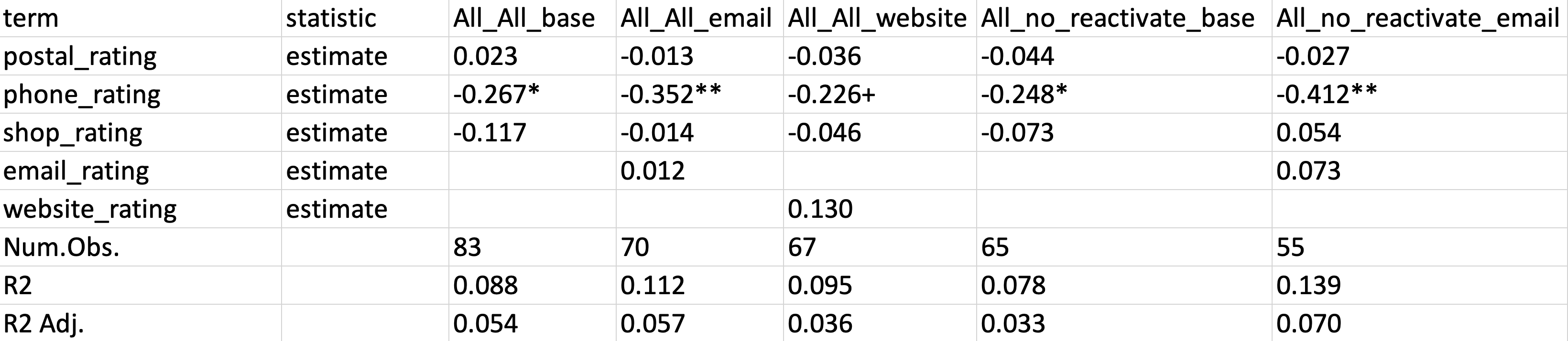
Examining the first few columns shows that not only the results print nicely, but they also include model names indicating the subgroups of each lm() call. Accepting a named list-columns of model objects is indeed a fantastic feature of the modelsummary() function.

The call to modelsummary() above gives us a quick and compact overview of our results in Excel. However, one minor issue is that the p-value stars appear in the same column as the model coefficients. For a better presentation and reporting, I prefer having the stars in a separate column. To achieve this, we can set the output argument to "data.frame", add the stars as statistic, convert the results to long format with pivot_wider() and save the resulting data.frame to Excel with openxlsx::write.xlsx(). Since this is a minor issue, I leave the code for the interested reader in the output box below.

out <- modelsummary(models = all_grid_upd_vars_form$mod,
                    output = "data.frame",
                    gof_omit = "AIC|BIC|Log.Lik|RMSE",
                    coef_omit = "(Intercept)",
                    statistic = "stars") |>
  mutate(statistic = ifelse(statistic == "", "estimate", statistic)) |>
  select(-part) |>
  pivot_wider(names_from = statistic,
              values_from = -c(term, statistic),
              values_fn = as.numeric)

openxlsx::write.xlsx(out, "model_results2.xlsx")

Endgame

With the building blocks introduced above, we can now combine everything and extend this approach even further.

Let’s say we want to compare two different versions of our dependent variable. The original variable and a collapsed top-box version csat_top taking 1 if a customer gave the best rating and 0 otherwise.

Again, we create a character vector holding the names of our dependent variables, dep_vars, and use it to expand our data-less grid from above.

csat_named_top <- csat_named |>
  mutate(csat_top = ifelse(csat == 5, 1, 0))

dep_vars <- c("csat", "csat_top")

all_grps_grid_final <- all_grid_upd_vars |>
  expand_grid(dep_vars)

all_grps_grid_final
#> # A tibble: 80 × 6
#>    product type  model_spec            filter_ls    update_vars  dep_vars
#>    <chr>   <chr> <chr>                 <named list> <named list> <chr>   
#>  1 All     All   base                  <lgl [1]>    <NULL>       csat    
#>  2 All     All   base                  <lgl [1]>    <NULL>       csat_top
#>  3 All     All   email                 <lgl [1]>    <chr [1]>    csat    
#>  4 All     All   email                 <lgl [1]>    <chr [1]>    csat_top
#>  5 All     All   website               <lgl [1]>    <chr [1]>    csat    
#>  6 All     All   website               <lgl [1]>    <chr [1]>    csat_top
#>  7 All     All   both                  <lgl [1]>    <chr [2]>    csat    
#>  8 All     All   both                  <lgl [1]>    <chr [2]>    csat_top
#>  9 All     All   both_plus_interaction <lgl [1]>    <chr [1]>    csat    
#> 10 All     All   both_plus_interaction <lgl [1]>    <chr [1]>    csat_top
#> # … with 70 more rows

Next, we update the formula, generate the data on the fly, calculate our model and prepare the results using ‘broom’. Note that we do all of this within just one call to dplyr::mutate(), since it allows us to define multiple columns and append them to our nested data.frame. Finally, we drop columns that we don’t need anymore.

all_grps_grid_final_res <- all_grps_grid_final |>

  rowwise() |>

  mutate(
    
  # dynamically name list
  form = list2( "{product}_{type}_{model_spec}_{dep_vars}" :=
  # update formula
    update(min_formula, # old formula
           reformulate(c(".", update_vars), dep_vars)) # changes to formula
  ),
    
  mod = list(
    lm(form,
  # create data on the fly
       data = filter(csat_named_top,
                     .env$product == "All" | .env$product == product,
                     eval(filter_ls)
       )
    )
  ),

  res = list(broom::tidy(mod)),

  modstat = list(broom::glance(mod))

  ) |>
  select(product:model_spec, dep_vars, mod:modstat)

all_grps_grid_final_res
#> # A tibble: 80 × 7
#> # Rowwise: 
#>    product type  model_spec            dep_vars mod    res              modstat 
#>    <chr>   <chr> <chr>                 <chr>    <list> <list>           <list>  
#>  1 All     All   base                  csat     <lm>   <tibble [4 × 5]> <tibble>
#>  2 All     All   base                  csat_top <lm>   <tibble [4 × 5]> <tibble>
#>  3 All     All   email                 csat     <lm>   <tibble [5 × 5]> <tibble>
#>  4 All     All   email                 csat_top <lm>   <tibble [5 × 5]> <tibble>
#>  5 All     All   website               csat     <lm>   <tibble [5 × 5]> <tibble>
#>  6 All     All   website               csat_top <lm>   <tibble [5 × 5]> <tibble>
#>  7 All     All   both                  csat     <lm>   <tibble [6 × 5]> <tibble>
#>  8 All     All   both                  csat_top <lm>   <tibble [6 × 5]> <tibble>
#>  9 All     All   both_plus_interaction csat     <lm>   <tibble [7 × 5]> <tibble>
#> 10 All     All   both_plus_interaction csat_top <lm>   <tibble [7 × 5]> <tibble>
#> # … with 70 more rows

As we add more complex functions to our workflow, we can see that the code gets pretty messy, and hard to debug. To keep the code clean and to allow for easier debugging we can tuck away the more complex parts of our code in customs functions. More details on this can be found in the info box below.

# define custom functions
update_min_form <- function(upvars, dpvars) { # update_vars, dep_vars
    update(min_formula, # old formula
           reformulate(c(".", upvars), dpvars) # changes to formula 
           ) 
}

linear_mod <- function(form, prodvar, filter_inp) {
      lm(form,
  # create data on the fly
       data = filter(csat_named_top,
                     prodvar == "All" | .data$product == prodvar,
                     eval(filter_inp)
       )
    )
}

all_grps_grid_final_res2 <- all_grps_grid_final |>
  rowwise() |>
  mutate(
    form = list2("{product}_{type}_{model_spec}_{dep_vars}" := 
                    update_min_form(update_vars, dep_vars)
  
    ),
    mod = list(linear_mod(form, product, filter_ls)),
    res = list(broom::tidy(mod)),
    modstat = list(broom::glance(mod))
  ) |>
  select(product:model_spec, dep_vars, mod:modstat)

all_grps_grid_final_res2
#> # A tibble: 80 × 7
#> # Rowwise: 
#>    product type  model_spec            dep_vars mod    res              modstat 
#>    <chr>   <chr> <chr>                 <chr>    <list> <list>           <list>  
#>  1 All     All   base                  csat     <lm>   <tibble [4 × 5]> <tibble>
#>  2 All     All   base                  csat_top <lm>   <tibble [4 × 5]> <tibble>
#>  3 All     All   email                 csat     <lm>   <tibble [5 × 5]> <tibble>
#>  4 All     All   email                 csat_top <lm>   <tibble [5 × 5]> <tibble>
#>  5 All     All   website               csat     <lm>   <tibble [5 × 5]> <tibble>
#>  6 All     All   website               csat_top <lm>   <tibble [5 × 5]> <tibble>
#>  7 All     All   both                  csat     <lm>   <tibble [6 × 5]> <tibble>
#>  8 All     All   both                  csat_top <lm>   <tibble [6 × 5]> <tibble>
#>  9 All     All   both_plus_interaction csat     <lm>   <tibble [7 × 5]> <tibble>
#> 10 All     All   both_plus_interaction csat_top <lm>   <tibble [7 × 5]> <tibble>
#> # … with 70 more rows

Although we are not specifically interested in the results, below is one way to filter out those models that are statistically significant at the 10% level arranged by adjusted r-squared in descending order:

all_grps_grid_final_res |>
  unnest(modstat) |>
  select(-c(sigma, statistic, df:df.residual)) |>
  filter(p.value < 0.1) |>
  arrange(desc(adj.r.squared))
#> # A tibble: 4 × 10
#>   product  type     model…¹ dep_v…² mod   res      r.squ…³ adj.r…⁴ p.value  nobs
#>   <chr>    <chr>    <chr>   <chr>   <lis> <list>     <dbl>   <dbl>   <dbl> <int>
#> 1 advanced no_reac… base    csat_t… <lm>  <tibble>  0.423   0.279   0.0765    16
#> 2 advanced All      base    csat_t… <lm>  <tibble>  0.349   0.234   0.0575    21
#> 3 All      All      email   csat    <lm>  <tibble>  0.112   0.0575  0.0973    70
#> 4 All      All      base    csat    <lm>  <tibble>  0.0884  0.0538  0.0613    83
#> # … with abbreviated variable names ¹​model_spec, ²​dep_vars, ³​r.squared,
#> #   ⁴​adj.r.squared

Wrap-up

That’s it! This post started out easy and got quite complex in the end. I hope to have shown how the original Many Models Approach can be refined from running the same model on various distinct subsets of data to running different variations of a model on many partly overlapping subsets. I hope you enjoyed this post. If you use other helper functions or have a better approach for calculating many models, I’d love to hear your feedback. Feel free to share your thoughts in the comments below or via Twitter, Mastodon, or GitHub.

Acknowledgements

I’m thankful for the many comments I have received for the initial version of this blog post. Isabelle Ghement was so kind to provide in-depth feedback which helped me to, hopefully, explain some of the concepts more concisely. Many thanks for that!

#> ─ Session info ───────────────────────────────────────────────────────────────
#>  setting  value
#>  version  R version 4.2.1 (2022-06-23)
#>  os       macOS Big Sur ... 10.16
#>  system   x86_64, darwin17.0
#>  ui       X11
#>  language (EN)
#>  collate  en_US.UTF-8
#>  ctype    en_US.UTF-8
#>  tz       Europe/Berlin
#>  date     2023-07-12
#>  pandoc   2.19.2 @ /Applications/RStudio.app/Contents/MacOS/quarto/bin/tools/ (via rmarkdown)
#> 
#> ─ Packages ───────────────────────────────────────────────────────────────────
#>  package      * version    date (UTC) lib source
#>  backports      1.4.1      2021-12-13 [1] CRAN (R 4.2.0)
#>  broom        * 1.0.1      2022-08-29 [1] CRAN (R 4.2.0)
#>  cachem         1.0.6      2021-08-19 [1] CRAN (R 4.2.0)
#>  cli            3.6.0      2023-01-09 [1] CRAN (R 4.2.0)
#>  digest         0.6.31     2022-12-11 [1] CRAN (R 4.2.0)
#>  downlit        0.4.2      2022-07-05 [1] CRAN (R 4.2.0)
#>  dplyover     * 0.0.8.9002 2022-10-15 [1] Github (timteafan/dplyover@f0cd984)
#>  dplyr        * 1.1.0      2023-01-29 [1] CRAN (R 4.2.0)
#>  ellipsis       0.3.2      2021-04-29 [1] CRAN (R 4.2.0)
#>  evaluate       0.19       2022-12-13 [1] CRAN (R 4.2.0)
#>  fansi          1.0.3      2022-03-24 [1] CRAN (R 4.2.0)
#>  fastmap        1.1.0      2021-01-25 [1] CRAN (R 4.2.0)
#>  fs             1.5.2      2021-12-08 [1] CRAN (R 4.2.0)
#>  generics       0.1.3      2022-07-05 [1] CRAN (R 4.2.0)
#>  glue           1.6.2      2022-02-24 [1] CRAN (R 4.2.0)
#>  highr          0.10       2022-12-22 [1] CRAN (R 4.2.0)
#>  htmltools      0.5.4      2022-12-07 [1] CRAN (R 4.2.0)
#>  hugodownplus   0.0.0.9000 2023-02-19 [1] Github (timteafan/hugodownplus@d79c4c0)
#>  knitr          1.41       2022-11-18 [1] CRAN (R 4.2.0)
#>  lifecycle      1.0.3      2022-10-07 [1] CRAN (R 4.2.0)
#>  magrittr       2.0.3      2022-03-30 [1] CRAN (R 4.2.0)
#>  memoise        2.0.1      2021-11-26 [1] CRAN (R 4.2.0)
#>  modelsummary * 1.3.0      2023-01-05 [1] CRAN (R 4.2.0)
#>  openxlsx       4.2.5.2    2023-02-06 [1] CRAN (R 4.2.0)
#>  pillar         1.8.1      2022-08-19 [1] CRAN (R 4.2.0)
#>  pkgconfig      2.0.3      2019-09-22 [1] CRAN (R 4.2.0)
#>  purrr        * 1.0.1      2023-01-10 [1] CRAN (R 4.2.0)
#>  R6             2.5.1      2021-08-19 [1] CRAN (R 4.2.0)
#>  Rcpp           1.0.9      2022-07-08 [1] CRAN (R 4.2.0)
#>  rlang        * 1.0.6      2022-09-24 [1] CRAN (R 4.2.0)
#>  rmarkdown      2.19       2022-12-15 [1] CRAN (R 4.2.0)
#>  rstudioapi     0.14       2022-08-22 [1] CRAN (R 4.2.0)
#>  sessioninfo    1.2.2      2021-12-06 [1] CRAN (R 4.2.0)
#>  stringi        1.7.8      2022-07-11 [1] CRAN (R 4.2.0)
#>  stringr        1.5.0      2022-12-02 [1] CRAN (R 4.2.0)
#>  tables         0.9.10     2022-10-17 [1] CRAN (R 4.2.0)
#>  tibble         3.1.8      2022-07-22 [1] CRAN (R 4.2.0)
#>  tidyr        * 1.2.1      2022-09-08 [1] CRAN (R 4.2.0)
#>  tidyselect     1.2.0      2022-10-10 [1] CRAN (R 4.2.0)
#>  utf8           1.2.2      2021-07-24 [1] CRAN (R 4.2.0)
#>  vctrs          0.5.2      2023-01-23 [1] CRAN (R 4.2.0)
#>  withr          2.5.0      2022-03-03 [1] CRAN (R 4.2.0)
#>  xfun           0.36       2022-12-21 [1] CRAN (R 4.2.0)
#>  yaml           2.3.6      2022-10-18 [1] CRAN (R 4.2.0)
#>  zip            2.2.2      2022-10-26 [1] CRAN (R 4.2.0)
#> 
#>  [1] /Library/Frameworks/R.framework/Versions/4.2/Resources/library
#> 
#> ──────────────────────────────────────────────────────────────────────────────